0%

RL knowledge List {.collection-title}

Name Tags keypoints


Value of the action W1_MAB Value of action = expected reward when the action is taken, q * (a) are defined as the expectedreward R_t from the action A_t but q*(a) we dont know→ we need to estimate it
Sample-Average Method W1_MAB Q_t(a) are defined as (sum of rewards when a taken prior to t)/(number of times a taken prior to t),
the doctor example W1_MAB As the doctor observe more patients, the estimated approach the true action value (**the sample average method**)
Action Selection W1_MAB The greedy action → they think it currently is the best! → has the largest estimated action value The agent is trying to get the most reward it can!
Balance W1_MAB short-term reward: choose greedy action → gamma = 0, not thinking about future at all long term reward: choose non-greedy action→ sacrifice immediate reward→ hopping to get more information about other actions → gamma = 1, thinking about future gamma: discount factor
Exploration- exploitation Dilemma W1_MAB conflict? balance?
Estimate action value incrementally W1_MAB Web advertisement problem
Incremental Update Rule Q_n+1 ⇒ 1/n * Sum(Ri)| i = 1 to n ⇒ 1/n *(R_n+ Sum(Ri)| i = 1 to n-1) Q_n+1 = Q_n + ( Rn -Q_n)/n**New Estimate ← Old Estimate + StepSize (Target -OldEstimate)*
Non- stationery Bandit Problem W1_MAB ???
What is the Trade Off W1_MAB Exploration: improve knowledge for long term benefit Exploitation: exploit short term benefit WE can not do both simultaneously
Epsilon-Greedy Action Selection W1_MAB ROLL a DICE epsilon: the possibility of choosing to explore
Optimistic Initial Values W1_MAB encourage exploration in early steps
Upper Confidence Bound Action Selection W1_MAB UCB = Upper Confidence Bound Use to decide the Action Selection Process,**betweenExploration&ExploitationHow UCB action-selection usesuncertaintyinestimationto drive exploration**
The difference of MAB and MDP W2_MDP MAB: same situation at each time→ single state→ the same action is always optimal MDP: different situation→ different response→ action chosen affect the amount of reward we can get into the future
Example W2_MDP Bandit algorithm tells a policy(which treatment to choose) for each trial. If he choose the sub optimalmedicine (i.e., performance of the medicine is less than other one) to treat the patient, then the cumulative performance will decrease. Unlike bandit, In MDP when you take an action, you will be in different state. MAB = MDP with**singlestateSituation = state, the action A_t change the state in MDP, create a new state St+1**
What is MDP? W2_MDP carrot / other vegetable , but different situation calls for different reactions carrot(lion) think about long term impact of our decisions
How to represent the dynamics of an MDP W2_MDP dynamics , transition dynamics from one state → to another
Formalization of MDP W2_MDP MDP formalization is flexible and abstract. \
states can be low level abstraction or high level abstractions, so it can be usde in various usages. (e.g. pixels, or object description in a photo) * time step can be short or very large
What’s the relationship of MDP and RL? W2_MDP RL : solve control task or prediction task MDP: sequential decision making problems, forma lize a wide range of this problems
RL W2_MDP RL: the goal for the agent is to maximize the future reward describe how the reward are related to the goal of the agent: long term goal, reward and future motion Returen Gt are defined as R_t+1 + R_t+2 + R_t+3 +… E(G) =E (sum(R…..)) maximize the expected Return → should be finite
identify episodic tasks W2_MDP naturally breaks into chucks called episodes each episode begins independently of how the previous one ends. e.g. Chess Game
What is a Reward Hypothesis? W2_MDP maximize the expected value expected future retuen That all of what we mean by goals and purposes can be well thought of as maximization of the expected value of the cumulative sum of a received scalar signal****(reward). Goals and purpose can be thought of as the maximization of the expected value of the cumulative sum of scalar rewards received
Continuing Tasks W2_MDP
Examples of Episodic and continuing tasks W2_MDP Epsodic: chess game regardless of how the game end, the new game states indepently
W2 summary W2_MDP MDP can formalize all problems in RL { State, Action, Rewards} Long term consequences, Actin → Future States + Rewards The Goal of RL: maximize**Total future reward → balance immediate reward with long term actions expected discounted sum of future rewards*
Discount W2_MDP 0<gamma <1 , the return remains finite gamma → 1, care about short term reward gamma→0 , we care about long term reward
Solve RL W2_MDP first step → MDP problems
Value Functions, Bellman Equations W3_Policy&Belman Once the problem is formulated as an MDP, finding theoptimal policy is more efficient when using value functions. This week, you will learn the definition of policies and value functions, as well as Bellman equations, which is the key technology that all of our algorithms will use.
Policy W3_Policy&Belman choose an action → reward + next state A policy is a distribution over actions for each possible state.
stochastic and deterministic policy W3_Policy&Belman Deterministic Policy: A Policy maps each states to a single action.**probability of 1** Policy(s) = a, States = s0, s1, s2 ; Actions = a0, a1, a2 (use Pie) Pi(s0) → a1, Pi(s1)→a0, Pi(s2)→a0. of course you can have same action for different state. In general, a policy assigns possibility to each action in each state. Pi(a|s) → represent a probability of selection of action a in state S Stochastic Policy: multi action be selected with non zero probability distribution → select actions in state S.**The stochastic policy might take the same step as the deterministic policy did.→ reach the Goal. Exploration/Exploitation trade-off (Epsilon greedy): can be useful for exploration**
generate examples of valide policies for MDP W3_Policy&Belman It is important that Policy only depends on the current state, not on thetime and previous state Valid policies:You don’t know about previous state anymore!!!!**You dont knowtime! Invalide Policies:The action depends on **something other than the state
Summary W3_Policy&Belman A policy maps**the current state**onto a set of possibilities for taking each action Policy only depends on the current state
Value Functions W3_Policy&Belman Delayed Reward: short term gain / long term gain? How to get a policy that achieve the most reward in the long term run? → Value Function is introduced to solve this issue.
Describe the role of state value/ action value function W3_Policy&Belman State Value Function: v(s) are defined as Expectation of (Future Reward an agent can expect to receive stating from a particular state) Action Value Function q_pi(s,a) are defined as Expected_pi (G_t | S_t =S, A_t = a) Value function predict rewards into the future
the relation between value functions and policies W3_Policy&Belman action, state, policy
examples of valid value function for a given MDP W3_Policy&Belman Chess game Reward : win +1; draw or loss 0 (not enough information to tell us how to achieve the goal) Value Function: Value V_pi(s) → probability for winning if we follow current policy Pi, at the current state
Bellman equation W3_Policy&Belman value of state and its possible successor derive Bellman equationstate value function / action value function Understand how Bellman equation relates →**current and future values V_pi(s) are defined as the E_pi (Gt| St = s)** and G_t = R_t + gamma \
G_t+1
Why Bellman equation W3_Policy&Belman we can only directly solve small DMP problems use Bellman equation, possible to solve chess problems, scale up to large problems
Optimal Policies W3_Policy&Belman Policy→ how an agent behave → Value Function What’s the goal of RL: We want to find the best policy in the long run! How to find → we can get different Value on different Policy →In some state, Policy had different value→ pi(1) ≥pi(2) iff line 1 isabove line 2 An optimal policy**PI*is that italways has the highest possible valuein every state. There’s alwaysat least one Optimal policy( maybe more)Proof: Pi(3) = Pi(1) , Pi(2) , Optimal → pi *⇒ alwasy exist optimal policy!!!!
How to find Optimal policy W3_Policy&Belman simple question→ Brute Force Search complex→how to optimize the search in the policy space?→ Bellman Optimality Equations
W3 Summary W3_Policy&Belman what is a policy→ current state → tell an agent how to behave determinate: map sate → an action stochastic: map each state to a probability distribution value function on States and Actions, probability to win
The optimal state-value function: W3_Policy&Belman **Is unique in every finite MDP
The Bellman optimality equation is actually a system of equations, one for each state, so if there are N states, then there are N equations in N unknowns. If the dynamics of the environment are known, then in principle one can solve this system of equations for the optimal value function using any one of a variety of methods for solving systems of nonlinear equations. All optimal policies share the same optimal state-value function.
What is DP W4_DP Dynamic Programming function p can be used to solve Policy evaluation and Control problem
Policy Evaluation & Control W4_DP distinction between policy evaluation and control Control ⇒task of finding a policy to obtain as much as possible DP problems use Bellman equations to defineiterative algorithms for both policy evaluation and control
Policy Evaluation W4_DP How good pi is? → pi → V_pi pi, p,gamma → DP → v_pi optimal policy! Control task complete iff current policy = optimal policy V_pi → policy evaluation pi * → control algorithms → compute value → DP
Iterative Policy Evaluation W4_DP DP are working as turning Bellman Equation intoupdate rules. First algorithm in DP → Iterative Policy Algorithms equation → iterative → get a approximate value → closer and closer to the value function(updated rule)Each iterationS → Sweep →v_pi V_pi is the unique solution to the bellman Equations
Policy Improvements W4_DP
Policy Iteration W4_DP You randomly select a policy and find value function corresponding to it , then find a new (improved) policy based on the previous value function, and so on this will lead to optimal policy
sequential decision making problem W2_MDPsocrative Long-term goal are generally more importantthan short-term consequences Agent does not always know completely the state of the environment e.g., partial observable problems
MDP W2_MDPsocrative State Space Action Space One-Step Dynamics In continuing tasks the discount factor must be smaller than 1
Explain briefly what is the reward hypothesis W2_MDPsocrative The reward hypothesis says that the agent is going to maximize the value of expected value of the cumulative sum of the received reward on the current state
Bellman Expectation Equations W2_MDPsocrative allows to evaluate a policy might be computationaly infeasible for large problems requires the knowledge of one step dynamics
Why DP W4_DPsocrative solving MDP is not easy
Define sweep in Iterative Policy Evaluation socrative first we have an initial step to estimation the value of the policy, then we use an iterative approach to update an estimation for the policy evaluation function, So we have a V’_pi to update the V_pi value at eachk step**for all states = at eachiteration of the algorithm, itupdates the value functionfor all the states , it“sweeps” through the state spaceof the problem**
Untitled

Slides Review {.collection-title}

Name Tags Keypoints


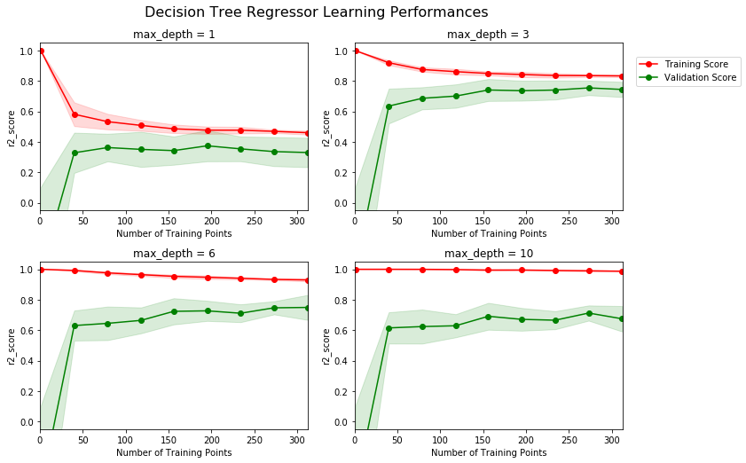
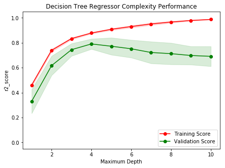
Bias-Variance Tradeoff 05_ModelEvaluation/Selection How to evaluate a model, can not use loss function The Bias-Variance is a framework to analyze the performance of models. 1. variancemeasures the difference between each model learned from a particular dataset and what we expect to learn. More sample / simpler model → decrease Variance 2. bias measures the difference betweentruth (𝑓) and what we expect to learn: more complex model→ decrease Bias
Model Assessment 05_ModelEvaluation/Selection high variance : under fitting high bias: overfitting low bias, low variance: good !
Regularization and Bias-Variance 05_ModelEvaluation/Selection The Bias-Variance decomposition explains why regularization allows to improve the error on unseen data.**Lasso outperforms Ridge regression when few features are related to the output*
Training Error/Prediction Error 05_ModelEvaluation/Selection Training Error: t_n-y(x_n) Prediction Error: (t_n-y(x_n)) \
p(x,t)
In practice 05_ModelEvaluation/Selection 1. Split randomly data into a training set and test set 2. Optimize model parameters using the training set 3. Estimate the prediction error using the test set high bias:training error is close to test error but they are both higher than expected high variance:training error is smaller than expected and it slowly approaches the test error
data split 05_ModelEvaluation/Selection Training Data → train model get parameter Validation Data→ validation error → select model with validation step → Test Data to estimate prediction error → raise 2 problems 1. enough validation data → less training data 2. overfitting ? How to solve ⇒ Cross Validation LOOCV ( lower bias but expensive to compute)/K-Fold cross validation (split in to K-folds, little bias, cheaper to compute)
How to choose the model 05_ModelEvaluation/Selection Reducing the variance choose right feature: the most effective subset of all the possible features dimensional reduction:lower- dimensional space Regularization: the values of the parameters are shrunked toward zero
No free lunch Theorems 05_ModelEvaluation/Selection Your favourite learner will not be always the best!
Feature Selection 05_ModelEvaluation/Selection AIC, BIC, AdjusterR2, etc. Cross-Validation
Dimensionality reduction 05_ModelEvaluation/Selection ⚠️Principal Component Analysis (PCA) P38**Dimensionality reduction aims at reducing the dimensions of input space, but it differs from feature selection in two major respects: it uses all the features and maps them into a lower-dimensionality space it is an unsupervised approach!*
Bagging and Boosting 05_ModelEvaluation/Selection \
Bootstrap Aggregation= Bagging(自主聚合)→ decrease high variance → suitable foe learner that is low bias and high variance/ overfitting problem ← bagging is suitable to decrease variance*** Boosting: high bias, the learner is not good enough ← need to fix it, boosting !!!!!!! → decrease bias/ still use simple learner/ keep the same variance (* still using weak learners: decision trees …) AdaBoost
VC dimension???? 06_LearningTheory ⚠️VC dimension
Kernel Ridge Regression 07_KernalMethods 看图片分布辨别用什么方法,linear/kernel
Kernel Design 07_KernalMethods
Kernel Regression 07_KernalMethods
Kernel Trick 07_KernalMethods can be used in …. Ridge Regression K-NN Regression Perceptron (Nonlinear) PCA Support Vector Machines … even Generative Models
What is MAB? 13_MAB Multi-arm bandit! far-sighted: gamma exploration/exploitation
different categories 13_MAB - Determistic - Stochastic { frequentist MAB , Bayesian }**-Adversarial Infinite time horizon: need to explore to gather more informationto find the best overall actionFinite time horizon: need tominimize short term lossbecauseuncertainty**
real example 13_MAB clinic test on new treatments! game playing slot machine Oil drilling new/unexplored/best/optimal
epsilon greeedy 13_MAB 1-e → greedy, instant reward; e → explore
softmax 13_MAB Weights the actions according to its estimated value Q(a|s) τ is a temperature parameter which decreases over time Even if these algorithms converge to the optimal choice, we do not know how much we lose during the learning process
MDP -relate to - MAB 13_MAB MDP → special case ( when the sate is single) → MAB State, Arm , Transition Matrix, Reward Function, discount factor(0< gamma <1 ), initial probability(optimistic estimation)
Goal 13_MAB maximize expectation value also minimize regret
Formulation 13_MAB 1. Frequentist formulation R(a1), . . . R(aN ) are unknown parameters A policy selects at each time step an arm based on the observation history 2. Bayesian formulation R(a1), . . . R(aN ) are random variables withprior distributions f1,…,fN A policy selects at each time step an arm based on the observation history and**on the provided priors**
Optimism in face of Uncertainty 13_MAB uncertain → explore→ get information & some loss in short term
Upper confidence Bound Approach 13_MAB ⭐️statistic approach → get a balance between exploration and exploitationthe bound length Bt(ai) depends on how much information we have on an arm, i.e., the number of times we pulled that arm so far Nt(ai)
UCB1 13_MAB ⭐️!!!!!!!!
Thompson Sampling 13_MAB 😇Pull the arm a with the highest sampled value Updatethe prior incorporating the new information Thompson Sampling → a method to solve MAB problem →optimal balance about explore/ exploit 1. sample from distribution to generate reward estimate 2. pick the arm with highest expectation 3. apply the arm and observe the reward 4. update distribution
EXP3 13_MAB 💥Variation of the Softmax algorithm Probability of choosing an arm,
Why DP 10_DP in order to find optimal policy of RL problem formulated in MDP, we need to find algorithms to evaluate policy value For small MDP problem→we can use brute force search For bigger MDP problem → DP can be used Dynamic Programming (DP) is a method that allow to solve a complex problem by breaking it down into**simpler sub-problems in a recursive manner** + Bellman Equation→ finite→unique Optimal solution→ pi*
Policy Evaluation 10_DP
Policy Improvement 10_DP
Policy Iteration 10_DP
Generalized Policy Iteration 10_DP
Efficiency of DP 10_DP
Untitled 12_TDL
What is supervised learning 02_SL It is the most popular and well established learning paradigm Data from an unknown function that maps an input 𝑥 to an output Goal: learn a good approximation of 𝑓 Classification if 𝑡 is discrete Regression if 𝑡 is continuous feature→ target Probability estimation if 𝑡 is a probability
When to apply supervised learning? 02_SL when human cannot perform the task When human can perform the task but cannot explain how When the task changes over time user-specific
overview 02_SL Define a loss function L Choose thehypothesis space H Find in H an approximation h of 𝑓 that minimizes L
Elements 02_SL Representation → Model Evaluation → Model selection Optimization →
Optimization 02_SL Combinatorial optimization e.g.: Greedy search ❑ Convex optimization e.g.: Gradient descent ❑ Constrained optimization e.g.: Linear programming
Parametric vs Nonparametric 02_SL Parametric:**fixed and finite number of parameters** Nonparametric: the number of parameters depends on the training set
Frequentist vs Bayesian 02_SL Frequentist: use probabilities to model the sampling processBayesian: use probability to model uncertainty about the estimate
Linear Regression 03_LR
Least Squares 03_LR
Regularization 03_LR
Least Squares and Maximum Likelihood 03_LR
Linear Classification 04_LC Learn, from a dataset 𝒟, an approximation of function 𝑓 𝑥 that maps input 𝑥 to a discrete class*𝐶
(with k = 1,…,𝐾)
Multi-class 04_LC In a multi-class problem we have K classes ❑ One-versus-the-rest approach uses K-1 binary cassifiers (i.e., that solve a two-class problem) each classifier discriminates 𝐶 and not 𝐶 regions ambiguity: region mapped to several classes ❑ One-versus-one approach uses K(K-1)/2 class binary classifiers each classifier discriminates between 𝐶 and 𝐶 𝑖𝑖 similary ambiguity of previous approach
hypothesis space 06_LearningTheory A hypothesis h is consistent with a training dataset 𝒟 of the concept c if and only if h(x) = c(x) for each training sample in 𝒟
VC Dimension 06_LearningTheory VC Dimension We define a dichotomy of a set S of instances as a partition of S into two disjoint subsets, i.e., labeling each instance in S as positive or negative ❑ We say that a set of instances S is shattered by hypothesis space H if and only if for every dichotomy of S there exists some hypothesis in H consistent with this dichotomy ❑ The Vapnik-Chervonenkis dimension, VC(H), of hypothesis space H over instance space X, is the largest finite subset of X shattered by H
Kernel Methods 07_KernalMethods Kernel methods allow to makelinear models work in nonlinear settings by mapping data tohigher dimensionswhere it exhibits linear patterns
Kernel in 1d example 07_KernalMethods linear separable
Kernel Functions 07_KernalMethods The kernel function is defined as the scalar product between the feature vectors of two data samples: Kernel function is symmetric:𝑘x,x′ =𝑘x′,x
sample-based methods 11_MonteCarlo With Dynamic Programming we are able to find theoptimal value function and the corresponding optimal policy
First-Visit & Evey-Visit 11_MonteCarlo Diff
Prediction & Control 11_MonteCarlo Diff Prediction: is to based on fixed policy to find maximize the estimation value of cumulated sum value. The input involves the policy Pi and MDP formulation. The output is the v_pi and q_pi Control: is to find be policy to achieve the goal, the policy is not fixed. The input is MDP description, and the output is the q_pi, V_pi, and Pi *(the optimal policy)
On-Policy & Off-Policy 11_MonteCarlo Diff policy iteration → how to get the Pivalue?
MC (Prediction and Control) 11_MonteCarlo Monte Carlo
diff between DP and MC 11_MonteCarlo ??
Valid Kernel 07_KernalMethods From the Mercers theorem, any continuous, symmetric, positive semi-definite kernel function can be expressed as a dot product in a high-dimensional space.
Rigid Regression, Logistic regression, Lasso Example What is it?
SVC sample Example 10^num_paramter, e.g. 100 = 10ˆ2
VC dimension Example
GMM Example GMM considers differently each dimension, by considering a generic covariance matrix while estimating the Gaussian distributions.
PARAMETRIC/NON–PARAMETRIC Example the difference
Q-learning Example what is q learning?

This semester I wrote a thesis for philosophy issue in Computer Science. At first, this was just a try in preparing for a master thesis next year. After following some lectures included in this course, I started to find more interest in writing a thesis in this field. My title is “Can computers write meaningful music?”, with the related fields of Computer Music, Music Composition, Computational Creativity, and Philosophy Issues in CS.

I am writing this note for the discussion session on next Tuesday.

Keypoints

  • Definition related: computers / computational creativity / programs to solve problems in music composition

  • Focus: Are they able to create music? Do they have the ability to create Meaningful muisic? Can computers have creativity?

  • Discussion in the Argument:

    • The definition of program → Arg 1. programs can do things beyond human expectations and limits{ Vague Problem, Unpredictable Answer, }

    • the definition of computational creativity

    • Stanford Encyclopedia of Philosophy

    • Judge the result, how human bias influence the result → Arg 2. Judging the composition itself { Definition of Creativity, Human Bias }

    • The essence of meaning {Expression of Emotions, Innovation Power}

    • Final conclusion

My reference

  • Literature Resource ( as supporting material)
  1. [1] Gérard Assayag et al. “Interaction with machine improvisation”. In:The Structure ofStyle. Springer, 2010, pp. 219–245.doi:10.1007/978-3-642-12337-5_10.

  2. [2] Simon Colton. “Creativity Versus the Perception of Creativity in Computational Sys-tems”. In:AAAI spring symposium: creative intelligent systems. Vol. 8. 2008.

  3. [3] Michael Edwards. “Algorithmic composition: computational thinking in music”. In:Communications of the ACM54.7 (2011), pp. 58–67.doi:10.1145/1965724.1965742.

  4. [4] Jose D Fernández and Francisco Vico. “AI methods in algorithmic composition: A com-prehensive survey”. In:Journal of Artificial Intelligence Research48 (2013), pp. 513–582.doi:10.1613/jair.3908.

  5. [5] Aaron Hertzmann. “Can computers create art?” In:Arts. Vol. 7. 2. MultidisciplinaryDigital Publishing Institute. 2018, p. 18.doi:10.3390/arts7020018.

  6. [6] MD Louis L. Lunsky. “Contemporary Approaches to Creative Thinking”. In:Arch In-tern Med112.2 (1963), pp. 300–301.doi:10.1001/archinte.1963.03860020198043.

  7. [7] Ramon Lopez de Mantaras and Josep Lluis Arcos. “AI and Music: From Compositionto Expressive Performance”. In:AI Magazine23.3 (2002), p. 43.

  8. [8] Marvin Minsky. “Why programming is a good medium for expressing poorly understoodand sloppily formulated ideas”. In: 1967, pp. 120–125.doi:10.1145/1094855.1094860.

  9. [9] David C Moffat and Martin Kelly. “An investigation into people’s bias against compu-tational creativity in music composition”. In:Assessment13.11 (2006).

  • Examples used:?

1. Music Information Retrieval

FILE: 1A. INTRODUCTION TO SOUND CLASSIFICATION

  • Slide 6 to 12
  • Slides 14 to 17
  • Slides 20 to 41
  • Slides 44 to 47
  • Slides 50 to 86
  • Slides 87 to 92

Classification

2. Computer Music Systems and Plugins

FILE: 2A. INTRODUCTION TO COMPUTER MUSIC ARCHITECTURES

• Slide 1 to 29

FILE: 2B.JUCE AS A PLATFORM FOR AUDIO PLUGINS

• Slides 4 and 5
• Slides 7 to 11

JUCE

3. SuperCollider

FILE: C.1 THE SUPERCOLLLIDER ECOSYSTEM

• Slides 3 to 48

SuperCollider

FILE: C.2 SUPERCOLLIDER AS A COMPUTER MUSIC LANGUAGE

• Slides 3 to 40
• Slides 47 to 68

C.2 SuperCollider

4. Music Interaction

FILE: D.1 INTRODUCTION TO MUSIC INTERACTION

• Slides 3 to 5

Intro to Music Interaction

FILE: D.2 MUSIC TRANSMISSION PROTOCOLS

• Slides 1 to 24
• Slides 27 to 36

• Slides 37 to 48

Music Transmission

FILE: D.3 USING MUSIC TRANSMISSION PROTOCOLS IN DIFFERENT CM ENVIRONMENTS

• Slides 1 to 53

Using music transmission

Today my friend come to lunch, lunch is prepared in the oven and I don’t want to move to take the timer.
Here is a way to set a timer on OSX.

‘’’
setalarm() {
sleep $(echo “$1 * 60” | bc)
say “Lunch Time”
}
setalarm 1
‘’’

What’s interesting

  • “say” command
  • say -v “voice name” “text to say”
  • voice name includes: Femal, Male and Novelty Voice, like “Cellos”, “Bad News”, “Pipe Organ”
  • output the recording: say -v “Cellos” “Lalalalalalalalala” -o save.aiff

Ps: supercollider 居然是 Beatles Paul Mccartney 的儿子在 1996 年开发的!

What is supercollider

  1. A platform for audio synthesis and algorithmic composition
  2. Users: musicians, artists, and researchers working with sound
  3. Three major components
    • scsynth:
      • a real time audio server
      • core
      • 400 + unit generators(“UGens”) of analysis, synthesis, and processing
      • known and unknown audio techniques
      • additive and subtractive synthesis, FM, granular synthesis, FFT, and physical modeling
* sclang: language
    - controls scsynth via Open Sound Control
    - algorithmic composition and sequencing
* scide: ide

Systems interfacing with SC

  1. send osc message from shell
  2. client using sc server
    Scheme, Smalltalk, Python, Processing, Perl, Java…

Processing

OSC Communication

Key points

  • concept: producing a behavior which is then interpreted by the user as demonstrating intelligent conversation
  • infer: without “understanding” (or “intentionality”), we cannot describe what the machine is doing as “thinking” and, since it does not think, it does not have a “mind” in anything like the normal sense of the word.
  • conclusion: the “strong AI” hypothesis is false.
  • Strong AI vs. biological naturalism: dk???

From the definition

  • How to understand a totally different thing from the concept?

  • How can we make computers to understand human emotions and human feelings

  • Even if a computer can do as human do, think as human thoughts, is it really on the same level of us?

  • How to learn Chinese from English dictionary?

  • What is the concept of computer programing?

  • If computers are set up a goal, we giving them abilities from executing programes, are they actually having to ability to do something, or they are just acting like humans while executing the programs.

  • If they pass the turing test, then it is human?

  • Is there real strong Artificial Intelligence?

  • All the doubts are not limiting the amount of intelligence a machine can display.

Other Doubts

  • What is the Turing test in music composition?
  • We can not tell which composition is made by human and which is made by machine?
  • If we find some music piece interesting, is it meaningful?
  • If we find some human composiiton boring and strange, is it meaningful?
  • What’s the border line between human composition and computer generated music if you can not tell the difference from listening to the music they made?
  • The intension, the passion and how much they want to convey through the emotional expression?
  • Human are social animals, so music is kind of connection? Music shoudl be meaningful in the social way?
  • What is art? Is it only the pursuit of human? Only human creation?
  • Artificial intelligence should be a human, able to understand and express emotion, then their works can be recognized as meaningful music.
  • Every music has its soul?

Reading

  1. “Minds, Brains, and Programs”,John Searle
  2. https://en.wikipedia.org/wiki/Chinese_room

0504 Music Interaction Design

What is interaction Design?

  • The practice of designing interactive digital products, environment

  • Who interact with who?
    machine, software, HCI

  • Where does interaction design enter in a computer music system?

    • gestures - input device
    • other IO Device, machine to machine
  • Setup an interaction

    • capture the gesture
    • mapping system
    • the transmission of the gestural and musical signals between different devices
    • Related areas: creative programming, electronics, telecommunication protocols
  • Example of M2M interaction

    • laptop orchestra by Stanford
    • position, gesture -> music parameters -> centre node -> synthesis -> music system (not a product, just used for this purpose)
    • IMU Motion Tracker(controller, feedback, flex sensors, connection with osc(?))
    • leap motion(device)
  • AI for music interaction

    • how if the computer could learn our way to interact with it?
    • eg. Wekinator, an AI system automatically study (gesture space -> music space)
  1. Deep Predictive Models in Interactive Music, https://arxiv.org/pdf/1801.10492.pdf

    • how is deep learning involved in music performace
    • especially digital musical instruments
    • musical predictions
    • difference between mapping and modelling
      • Mapping refers to connecting the control and sensing components of a musical instrument to parameters in the sound synthesis component
      • Modelling refers to capturing a representation of a musical process
  2. How to generate music?

    • ANN -> RNN -> LSTM : improved (to learn distant dependencies)
    • RNNs with LSTM cells were later used by Eck and Schmidhuber to generate blues music
    • generate music using Markov models to generate the emission probabilities of future notes based on those preceding
    • Bach music, polyphonic chorales of J. S. Bach have also been modelled by RNN
    • difference in these models ???
    • learn much about the temporal structure of music, and how melodies and harmonies can be constructed
    • Simon and Oore’s Performance RNN: goes further by generating dynamics and rhythmic expression, or rubato, simultaneously with polyphonic music.
    • WaveNet: producing samples
  3. Predictive models: instrument-level -> performer-level -> ensemble-level

Intro

1. High dimensional Feature

  • what is the difference between low dimensional feature and high dimensional feature
  • x = [x1,x2,…,xn] -> y
  • infinite dimensional features
  • select features based on the data

2. Regression vs Classification

  • regression: if y is continuous variable,
    e.g., price prediction
  • classification: if the label is a discrete variable
    e.g., the task of predicting the types of residence

3. Supervised learning in computer science

  • Image Classification: x = raw pixels of the picture, and y = label
  • Natural language processing

4. unsupervised learning

  • only have data without labels
  • goal is to find interesting structure in the data

5. Clustering & Other

  • k-mean clustering, mixture of Gaussians
  • clustering genes
  • principal component analysis (tools used in
    LSA)
  • word emeddings(Represent words by vectors),eg Word2vec
  • clustering words with similar meanings

6. Reinforcement Learning

  • learning to walk to the right
  • the algorithms can collect data interactively
  • method: try the strategy and collect feedbacks(Data Collections & Training),to improve the strategy based on the feedbacks

SL:Setup

  • Linear Regression
  • x -> y
  • gradient descent

Linear Algebra

Probability

Gaussian Discriminant Analysis

Support Vector Machines. Kernels.

Evaluation Metrics

Reference

  1. http://cs229.stanford.edu/notes2020spring/lecture1_slide.pdf
  2. http://cs229.stanford.edu/notes2020spring/cs229-notes1.pdf
  3. CS224N/CS231N
  4. Identifying Regulatory Mechanisms using Individual Variation Reveals Key Role for Chromatin Modification.
  5. Luo-Xu-Li-Tian-Darrell-M.’18

1. What is Machine Learning?

Two definitions of Machine Learning are offered.

  • Arthur Samuel described it as: “the field of study that gives computers the ability to learn without being explicitly programmed.” This is an older, informal definition.

  • Tom Mitchell provides a more modern definition: “A computer program is said to learn from experience E with respect to some class of tasks T and performance measure P, if its performance at tasks in T, as measured by P, improves with experience E.”

  • Example: playing checkers.
    E = the experience of playing many games of checkers
    T = the task of playing checkers.
    P = the probability that the program will win the next game.

  • In general, any machine learning problem can be assigned to one of two broad classifications: Supervised learning and Unsupervised learning.

  • Except from supervised learning and unsupervised, there are also Reinforcement learning, recommender systems.

用机器模拟人脑

  • 人可以描述问题,但不知道如何显式地解决问题
  • 让机器得到输入和输出,寻找解决途径
  • 计算机科学,可以应用在工业和基础科学上。{自动直升机,手写识别,自然语言,机器视觉,推荐算法}
  • 需要足够多的数据

不同类型的学习算法

  • 作为 Tools/methods, 选择哪一种方法要看得到的数据情况(离散的数据?连续的数据)和要解决的问题(预测?分类?)
  • 监督学习
  • 无监督学习
  • 强化学习

选择的问题

  • 需要理解算法本身,我们才能根据具体的实践问题,决定采用哪一种方法(最节省时间和精力)建立系统
  • 机器可以有多种方法达到目标,但是哪一种是最优的

分类问题

  • Classification: Discrete valued
  • Classification(discrete) CF Regression(Continus)

2. What is supervised learning

  • most important one in learning paradigm
  • an unknown function f that maps an input 𝑥 to an output t: D = {<x, t>}

Goal of SL

  • Goal: is to learn a good approximation of 𝑓
  • Input variables 𝑥 are usually called features or attributes
  • Output variables 𝑡 are also called targets or labels

Tasks

Classification if 𝑡 is discrete
Regression if 𝑡 is continuous
Probability estimation if 𝑡 is a probability

Elements in Supervised Learning

  1. Representation
    • Consist {linear models, instance-based, decision trees, set of rules, graphical models, neural networks, Gaussian Processes, Support vector machines, Model ensembles }
  2. Evaluation
    • {Accuracy, precision and recall, squared error, Likelihood,
      Posterior probability, Cost/Utility, Margin, Entropy, KL divergence}
  3. Optimization
    • { Combinatorial optimisation e.g.: Greedy search
      Convex optimisation e.g.: Gradient descent
      Constrained optimisation e.g.: Linear programming }

Process

  1. Training Set
  2. Learning Algorithms
  3. Function h(hypothesis) {Input: size of a house -> h -> Output:estimated price}

3. Unsupervised Learning

  • Unsupervised learning allows us to approach problems with little or no idea what our results should look like. We can derive structure from data where we don’t necessarily know the effect of the variables.
  • We can derive this structure by clustering the data based on relationships among the variables in the data.
  • With unsupervised learning there is no feedback based on the prediction results.

Example:

  • Clustering: Take a collection of 1,000,000 different genes, and find a way to automatically group these genes into groups that are somehow similar or related by different variables, such as lifespan, location, roles, and so on.

  • Non-clustering: The “Cocktail Party Algorithm”, allows you to find structure in a chaotic environment. (i.e. identifying individual voices and music from a mesh of sounds at a cocktail party).

4. Model and Cost Functions

  1. Linear Regression:

    • supervised learning:gives the “right answer” to the
    • Regression : predict real-valued output
      • Classification: get discrete-valued output {eg:0,1}
  2. Traning Models

    • number of training examples
    • input variables/ features
    • output variables/ target
  3. Workflow

    • Training Set ->Learning Algorithms ->

5. Linear Regression

6. Linear Classification

7. Model Evaluation, Selection Ensembles

Bias Variance

  1. The Bias-Variance is a framework to analyze the performance of models
  2. Definition:
    • data
    • model
    • performance
    • Thus we can decompose the expectected square error as:
  3. Model Variance,
  4. Case Study: Bias Variance for K-NN

我们希望模型准确,误差尽可能的小。

…….

8. Reference

  1. Material of prof. Marcello Restelli
  2. Pattern Recognition and Machine Learning, Bishop [PRML]
  3. Elements of Statistical Learning, Hastie et al. [ESL]
  4. Introduction to Statistical Learning, James et al. [ISL]
  5. The Lack of A Priori Distinctions Between Learning Algorithms, Wolpert, 1996

机器学习实验项目_波士顿房价预测

0. 项目背景

这是一个几年之前的机器学习练习项目。数据来源是UCI的机器学习知识库数据集。该数据从1978年开始,共506个数据点,涵盖了马萨诸塞州波士顿郊区的房屋信息数据。

在此项目中,我会使用这些数据训练并测试一个可用的预测模型,并对模型的性能和预测能力进行测试。训练好的模型可以对房屋的价值进行预测,对某些工作中,应用这个模型可以帮助他们了解房屋的潜在价值,是非常实用的。

从学习的角度来看,做这个项目则是可以初步了解机器学习的实践方法,了解如何处理数据,并熟悉 python 和 sklearn在项目中的使用。

提示:Code 和 Markdown 区域可通过 Shift + Enter 快捷键运行。此外,Markdown可以通过双击进入编辑模式。


1. 导入数据

本项目的数据集来自UCI机器学习知识库(数据集已下线)
可以看到,波士顿房屋这些数据于1978年开始统计,共506个数据点,涵盖了麻省波士顿不同郊区房屋14种特征的信息。
在此,首先我将针对本项目对原始数据集做以下处理:观察数据 -> 移除异常值 -> 思考哪些是和目标相关的特征。
具体处理如下:

  • 有16个'MEDV' 值为50.0的数据点被移除。 因为这些数据点包含遗失或者不明确的数值。
  • 有1个数据点的 'RM' 值为8.78. 这是一个异常值,已经被移除。
  • 对于本项目,房屋的'RM''LSTAT''PTRATIO'以及'MEDV'特征是必要的,其余不相关特征已经被移除。
  • 'MEDV'特征的值已经过必要的数学转换,可以反映35年来市场的通货膨胀效应。

运行下面区域的代码后,我就可以载入波士顿房屋数据集,以及一些此项目所需的Python库。
我会从 csv 文件中读取到需要的数值,如果成功返回数据集的大小,则表示数据集已载入成功。

1
2
3
4
5
6
7
8
9
10
11
12
# import 
import numpy as np
import pandas as pd
import visuals as vs # import supplement

# check Python version
from sys import version_info
if version_info.major != 2 and version_info.minor != 7:
raise Exception('Please use Python 2.7')

# show result in notebook
%matplotlib inline
1
2
3
4
5
6
7
# 载入波士顿房屋的数据集
data = pd.read_csv('housing.csv')
prices = data['MEDV']
features = data.drop('MEDV', axis = 1)

# 完成
print "Boston housing dataset has {} data points with {} variables each.".format(*data.shape)
Boston housing dataset has 489 data points with 4 variables each.

2. 分析数据

我需要继续观察目前得到的数据,以便在后续阶段能够理解对数据进行分析后得到的结果或对结果进行分析。

由于我的最终目标是将实现一个表现良好的房屋价值预估的模型,所以我依然需要把完整的数据集分成featuretarget

  • 特征'RM''LSTAT',和 'PTRATIO'
  • 目标变量'MEDV',是我希望预测的变量。

我用 featuresprices两个变量进行存储。

2.1 基础统计运算

我导入了numpy 执行计算。这些统计数据对于分析模型的预测结果非常重要的。

  • 计算prices中的'MEDV'的最小值、最大值、均值、中值和标准差;
  • 将运算结果储存在相应的变量中。
1
2
3
4
5
6
7
8
9
10
11
12
13
14
15
16
17
18
19
20
21
22
23

#目标:计算价值的最小值
minimum_price = np.min(prices)

#目标:计算价值的最大值
maximum_price = np.max(prices)

#目标:计算价值的平均值
mean_price = np.mean(prices)

#目标:计算价值的中值
median_price = np.median(prices)

#目标:计算价值的标准差
std_price = np.std(prices)

#目标:输出计算的结果
print "Statistics for Boston housing dataset:\n"
print "Minimum price: ${:,.2f}".format(minimum_price)
print "Maximum price: ${:,.2f}".format(maximum_price)
print "Mean price: ${:,.2f}".format(mean_price)
print "Median price ${:,.2f}".format(median_price)
print "Standard deviation of prices: ${:,.2f}".format(std_price)
Statistics for Boston housing dataset:

Minimum price: $105,000.00
Maximum price: $1,024,800.00
Mean price: $454,342.94
Median price $438,900.00
Standard deviation of prices: $165,171.13

2.2 特征观察

如前文所述,本项目中我们关注的是其中三个值:'RM''LSTAT''PTRATIO',对每一个数据点:

  • 'RM' 是该地区中每个房屋的平均房间数量;
  • 'LSTAT' 是指该地区有多少百分比的业主属于是低收入阶层(有工作但收入微薄);
  • 'PTRATIO' 是该地区的中学和小学里,学生和老师的数目比(学生/老师)。

凭直觉,上述三个特征中对每一个来说,你认为增大该特征的数值,'MEDV'的值会是增大还是减小呢?

  • RM 变大,MEDV 越大,因为房间多整体空间更大
  • LSTAT 越大,MEDV 越小,因为代表着当地经济价值比较低
  • PTRATIO 越大,MEDV 越低,因为该地区学生多教师少,教育价值降低了

2.2 数据分割与重排

接下来,我需要把波士顿房屋数据集分成训练和测试两个子集。
通常在这个过程中,数据也会被重排列,以消除数据集中由于顺序而产生的偏差。

我使用 sklearn.model_selection 中的 train_test_split, 将featuresprices的数据都分成用于训练的数据子集和用于测试的数据子集。

  • 分割比例为:80%的数据用于训练,20%用于测试;
  • 选定一个数值以设定 train_test_split 中的 random_state ,这会确保结果的一致性;
1
2
3
# 提示: 导入train_test_split
from sklearn.model_selection import train_test_split
X_train, X_test, y_train, y_test = train_test_split(features, prices, test_size=0.2, random_state=22)

2.3 训练及测试

将数据集按一定比例分为训练用的数据集和测试用的数据集对学习算法有什么好处?

如果用模型已经见过的数据,例如部分训练集数据进行测试,又有什么坏处? 如果没有数据来对模型进行测试,会出现什么问题?

  • 将数据集按照一定比例分割,我们可以合理评估学习算法在面对未知数据时的表现效果
  • 用来评价模型的数据如果不是独立于样本的,则可能评价结果是不准确的情况。我们也无法得出,这个算法是否可以应用在更广泛的情况

3. 模型衡量标准

在项目的第三步中,你需要了解必要的工具和技巧来让你的模型进行预测。用这些工具和技巧对每一个模型的表现做精确的衡量可以极大地增强你预测的信心。

3.1 定义衡量标准

如果不能对模型的训练和测试的表现进行量化地评估,就很难衡量模型的好坏。一般情况下,我们可以定义一些衡量标准,这些标准可以通过对某些误差或者拟合程度的计算来得到。在这个项目中,你将通过运算决定系数 R2 来量化模型的表现。模型的决定系数是回归分析中十分常用的统计信息,经常被当作衡量模型预测能力好坏的标准。

R2的数值范围从0至1,表示目标变量的预测值和实际值之间的相关程度平方的百分比。一个模型的R2 值为0还不如直接用平均值来预测效果好;而一个R2 值为1的模型则可以对目标变量进行完美的预测。从0至1之间的数值,则表示该模型中目标变量中有百分之多少能够用特征来解释。模型也可能出现负值的R2,这种情况下模型所做预测有时会比直接计算目标变量的平均值差很多。

在下方代码的 performance_metric 函数中,我实现了:

  • 使用 sklearn.metrics 中的 r2_score 来计算 y_truey_predict的R2值,作为对其表现的评判。
  • 将他们的表现评分储存到score变量中。

或(:这个并没有实现:)

  • (可选) 不使用任何外部库,参考决定系数的定义进行计算,这也可以帮助你更好的理解决定系数在什么情况下等于0或等于1。
1
2
3
4
5
6
7
8
9
# 导入r2_score
from sklearn.metrics import r2_score

def performance_metric(y_true, y_predict):
"""计算并返回预测值相比于预测值的分数"""

score = r2_score(y_true, y_predict)

return score
1
2
3
4
5
6
7
8
# 不导入任何计算决定系数的库

def performance_metric2(y_true, y_predict):
"""计算并返回预测值相比于预测值的分数"""

score = None

return score

3.2 拟合程度

假设一个数据集有五个数据且一个模型做出下列目标变量的预测:

真实数值 预测数值
3.0 2.5
-0.5 0.0
2.0 2.1
7.0 7.8
4.2 5.3

怎么样可以判断,这个模型已成功地描述了目标变量的变化?

通过运行下方的代码,我可以使用performance_metric函数来计算模型的决定系数。

1
2
3
# 计算这个模型的预测结果的决定系数
score = performance_metric([3, -0.5, 2, 7, 4.2], [2.5, 0.0, 2.1, 7.8, 5.3])
print "Model has a coefficient of determination, R^2, of {:.3f}.".format(score)
Model has a coefficient of determination, R^2, of 0.923.
  • 这个模型以及较为成功地描述了目标变量的变化。
  • 因为可以看到 R^2 计算结果为 0.923 意味着数据超过90的部分能够使用模型进行特征的描述和预测

4. 分析模型的表现

在项目的第四步,可以来看一下不同参数下,模型在训练集和验证集上的表现。
我只是用了一个特定的算法(带剪枝的决策树),在参数选择上,这个算法只包括了选择参数 'max_depth'
我会用全部训练集训练,但选择不同'max_depth' 参数,观察这个参数的变化如何影响模型的表现。
最后,画出模型的表现来对于分析过程十分有益,这可以让我直观地看到模型的表现。

4.1 学习曲线

  • 下方区域内的代码可以输出四幅图像,他们分别表现了一个决策树模型在不同最大深度下的表现。
  • 每一条曲线都直观得显示了随着训练数据量的增加,模型学习曲线的在训练集评分和验证集评分的变化。
  • 评分使用决定系数R2。曲线的阴影区域代表的是该曲线的不确定性(用标准差衡量)。
1
2
# 根据不同的训练集大小,和最大深度,生成学习曲线
vs.ModelLearning(X_train, y_train)

png

4.2 对学习曲线的观察

所以从上面的图形中,我应该怎么决定合适的最大深度呢?

其次,随着寻来拿数据量的增加,训练集曲线的评分正在发生变化,验证集曲线也有变化。我也需要考虑数据继续增加的情况下,如何保持或者有效提升模型的表现呢?但是学习曲线看上去最终都很稳定,是不是会最终收敛到一个特定的值。

  • 我想选择 max = 3,也就是将深度设定为3.
  • 从曲线的观察上来看,随着训练数据量的增加,训练集曲线评分降低了一点,但趋于稳定。
  • 随着训练数据量的增加,验证集曲线迅速上升后也趋于稳定
  • 如果有更多训练数据,且新训练数据分布和现有相同,模型的表现不会有什么明显提升,因为现在已经能够捕捉数据的全部特征了。

4.3 复杂度曲线

下列代码内的区域会输出一幅图像,用于展示了一个已经经过训练和验证的决策树模型在不同最大深度条件下的表现。

这个图形将包含两条曲线,一个是训练集的变化,一个是验证集的变化。跟学习曲线相似,阴影区域代表该曲线的不确定性,模型训练和测试部分的评分都用的 performance_metric 函数。

1
2
# 根据不同的最大深度参数,生成复杂度曲线
vs.ModelComplexity(X_train, y_train)

png

4.4 偏差(bias)与方差(variance)之间的权衡取舍

当模型以最大深度 1训练时,模型的预测是出现很大的偏差还是出现了很大的方差?当模型以最大深度10训练时,情形又如何呢?图形中的哪些特征能够支持你的结论?

我要如何判断模型是否出现了偏差很大或者方差很大的问题?

  • 模型深度为 1 时,偏差大。
  • 因为可以看到模型预测在训练集上的得分低,说明模型预测不准确。
  • 而当模型深度为 10 时,方差大。
  • 可以看到模型预测在训练集上的得分高,接近1,说明预测准确。但模型在训练集上表现较好,但测试集上表现差,说明面对新数据时表现不好。

4.5 最优模型的猜测

我应该选择哪一个最大深度,才能对未来(未知)的数据进行预测。

  • 按照图 5 来看可以选择深度为 6 的模型。
  • 个人认为,深度为 4 时,方差最小,但偏差仅仅超过0.8。
  • 随着深度增加,偏差仍在迅速缩小,而在 6 之后,偏差开始趋于稳定,处在0.9左右。
  • 此时方差看上去增大了0.1左右,可以接受。

5. 选择最优参数

5.1 网格搜索(Grid Search)

什么是网格搜索法?如何用它来优化模型?

  • 网格搜索,是一种系统地遍历多种参数组合,通过交叉验证确定最佳效果参数的方法
  • 使用网格搜索优化模型,可以对不同参数组合进行评估,得到最合适的参数组合,优化模型

5.2 交叉验证

  • 什么是K折交叉验证法(k-fold cross-validation)?
  • GridSearchCV是如何结合交叉验证来完成对最佳参数组合的选择的?
  • GridSearchCV中的'cv_results_'属性能告诉我们什么?
  • 网格搜索时如果不使用交叉验证会有什么问题?交叉验证又是如何解决这个问题的?

在下面 fit_model函数最后加入 print pd.DataFrame(grid.cv_results_) 可以查看更多信息。

  1. 什么是K折交叉验证法(k-fold cross-validation)?

    • K折交叉验证,是将训练数据(验证集)平分到 k 个容器。在每次实验时,选择其中 1 个容器中的数据作为验证集,其他(k-1)个容器作为训练集。
    • 继续训练模型,并进行验证。
    • 交叉验证会在过程中进行 k 次实验,然后取得 k 次实验测试结果的平均值。
  2. 网格搜索如何结合交叉验证完成最佳参数选择?

    • 这种方法中我们对每 1 个参数组合进行 1 次 K 折较差验证,得到平均分数。
    • 一般选择均分最高的参数组合作为最优参数,但如果品分标准是loss,会选择评分最低的参数组合。
  3. cv_results_属性代表什么?

    • cv_results_可以用来来获得最优参数组合
    • 它返回了一个字典,其中记录了每一组网格参数每一次实验时的结果,如时间、评估值、其他统计信息
  4. 网格搜索时如果不使用交叉验证会有什么问题?交叉验证又是如何解决这个问题的?

    • 网格搜索不使用交叉验证时所花费的训练时间更短,但模型参数并不是最优;
    • 交叉验证进行更多次的试验,使用了全部训练集,能够对每一个参数组合得出更准确的评分。

5.3 决策树算法

下面,我会使用决策树算法训练一个模型。

为了得出的是一个最优模型,我需要使用网格搜索法训练模型,以找到最佳的 'max_depth' 参数。我可以把'max_depth' 参数理解为决策树算法在做出预测前,可以允许的对数据提出问题的数量。而决策树也是监督学习算法中的一种。

在下方 fit_model 函数中,我进行了如下的定义:

  1. 定义 'cross_validator' 变量: 使用 sklearn.model_selection 中的 KFold 创建一个交叉验证生成器对象;
  2. 定义 'regressor' 变量: 使用 sklearn.tree 中的 DecisionTreeRegressor 创建一个决策树的回归函数;
  3. 定义 'params' 变量: 为 'max_depth' 参数创造一个字典,它的值是从1至10的数组;
  4. 定义 'scoring_fnc' 变量: 使用 sklearn.metrics 中的 make_scorer 创建一个评分函数;
    ‘performance_metric’ 作为参数传至这个函数中;
  5. 定义 'grid' 变量: 使用 sklearn.model_selection 中的 GridSearchCV 创建一个网格搜索对象;将变量'regressor', 'params', 'scoring_fnc''cross_validator' 作为参数传至这个对象构造函数中;

关于python函数的默认参数定义和传递,可以参考的资料是,这个MIT课程的视频

1
2
3
4
5
6
7
8
9
10
11
12
13
14
15
16
17
18
19
20
21
22
23
#提示: 导入 'KFold' 'DecisionTreeRegressor' 'make_scorer' 'GridSearchCV' 
from sklearn.model_selection import KFold,GridSearchCV
from sklearn.tree import DecisionTreeRegressor
from sklearn.metrics import make_scorer

def fit_model(X, y):
""" 基于输入数据 [X,y],利于网格搜索找到最优的决策树模型"""

cross_validator = KFold(n_splits=10)

regressor = DecisionTreeRegressor()

params = {'max_depth':range(1,11)}

scoring_fnc = make_scorer(performance_metric)

grid = GridSearchCV(regressor, params, scoring=scoring_fnc,cv=cross_validator)

# 基于输入数据 [X,y],进行网格搜索
grid = grid.fit(X, y)

# 返回网格搜索后的最优模型
return grid.best_estimator_

5.4 训练最优模型(*没有实现)

另外一种方法是在下方 fit_model 函数中:

  • 遍历参数‘max_depth’的可选值 1~10,构造对应模型
  • 计算当前模型的交叉验证分数
  • 返回最优交叉验证分数对应的模型

但这一个方法还没有完成。

1
2
3
4
5
6
7
8
9
10
11
12
13
14
15
16
17
18
19
20
# Not finished!

'''
不允许使用 DecisionTreeRegressor 以外的任何 sklearn 库

提示: 你可能需要实现下面的 cross_val_score 函数

def cross_val_score(estimator, X, y, scoring = performance_metric, cv=3):
""" 返回每组交叉验证的模型分数的数组 """
scores = [0,0,0]
return scores
'''

def fit_model2(X, y):
""" 基于输入数据 [X,y],利于网格搜索找到最优的决策树模型"""

#最优交叉验证分数对应的最优模型
best_estimator = None

return best_estimator

5.5 最优模型

最优模型的最大深度(maximum depth)是多少?

通过下面的代码,我能够将决策树回归函数代入训练数据的集合,以得到最优化的模型。并得到最大深度。

1
2
3
4
5
# 基于训练数据,获得最优模型
optimal_reg = fit_model(X_train, y_train)

# 输出最优模型的 'max_depth' 参数
print "Parameter 'max_depth' is {} for the optimal model.".format(optimal_reg.get_params()['max_depth'])
Parameter 'max_depth' is 4 for the optimal model.

可以看到,此时的最大深度为4,和我开始目测的不同。

6. 做出预测

当我们用数据训练出一个模型,它现在就可用于对新的数据进行预测。在决策树回归函数中,模型已经学会对新输入的数据提问,并返回对目标变量的预测值。你可以用这个预测来获取数据未知目标变量的信息,这些数据必须是不包含在训练数据之内的。

6.1 预测销售价格

接下来由于模型已经得到了,我需要开始应用这个模型处理一些问题。

假设我是一个在波士顿地区的房屋经纪人,我可以使用此模型以帮助你的客户评估他们想出售的房屋。

假设你已经从你的三个客户收集到以下的资讯:

特征 客戶 1 客戶 2 客戶 3
房屋内房间总数 5 间房间 4 间房间 8 间房间
社区贫困指数(%被认为是贫困阶层) 17% 32% 3%
邻近学校的学生-老师比例 15:1 22:1 12:1

那么接下来,我需要给每位客户的房屋销售的价格进行建议?并通过房屋特征的数值提供对于价格的合理判断。

运行下列的代码区域,我就可以使用优化的模型来为每位客户的房屋价值做出预测。并结合我在第一步中数据分析的阶段,计算出来的部分统计信息来辅助证明我的模型是否正确。

1
2
3
4
5
6
7
8
9
# 生成三个客户的数据
client_data = [[5, 17, 15], # 客户 1
[4, 32, 22], # 客户 2
[8, 3, 12]] # 客户 3

# 进行预测
predicted_price = optimal_reg.predict(client_data)
for i, price in enumerate(predicted_price):
print "Predicted selling price for Client {}'s home: ${:,.2f}".format(i+1, price)
Predicted selling price for Client 1's home: $409,100.00
Predicted selling price for Client 2's home: $285,600.00
Predicted selling price for Client 3's home: $957,218.18
  • 预测价值为409100、285600、957218 美元。

  • 从房屋特征来看,房屋质量的高中低档水平应该是 客户 3 (高档)> 客户 1 (中档)> 客户 2(低档) 。

  • 从统计数据来看,客户 1 的房屋价值处在 Min 与 Max 之间,接近均价和中位数。客户 2 的房屋价值较低,只稍微比 Min 高一点。客户 3 的房屋价值较高,接近 Max 价格。符合房屋特征的判断,因此预测还是是比较合理的。

6.2 使用模型进行预测

我对三个客户的房子的售价进行了预测。接下来,我会使用我的最优模型在整个测试数据上进行预测, 并计算相对于目标变量的决定系数 R2的值**。

1
2
3
4
5
6
7
8
9

# 提示:你可能需要用到 X_test, y_test, optimal_reg, performance_metric
# 提示:你可能需要参考问题10的代码进行预测
# 提示:你可能需要参考问题3的代码来计算R^2的值

from sklearn.metrics import r2_score
r2 = r2_score(y_test, optimal_reg.predict(X_test))

print "Optimal model has R^2 score {:,.2f} on test data".format(r2)
Optimal model has R^2 score 0.78 on test data

6.3 分析决定系数

刚刚计算了最优模型在测试集上的决定系数,但我应该如何评价这个结果?

结果为 0.78 结果不算太好,但也可以进行基本的房屋价值预测了。

6.4 模型的健壮性

一个最优的模型不一定是一个健壮模型。有的时候模型会过于复杂或者过于简单,以致于难以泛化新增添的数据;有的时候模型采用的学习算法并不适用于特定的数据结构;有的时候样本本身可能有太多噪点或样本过少,使得模型无法准确地预测目标变量。这些情况下我们会说模型是欠拟合的。

模型是否足够健壮来保证预测的一致性?

下面,我会采用不同的训练和测试集执行 fit_model 函数10次。

对一个特定的客户来说,预测是如何随训练数据的变化而变化的。

1
2
# 注释掉 fit_model 函数里的所有 print 语句
vs.PredictTrials(features, prices, fit_model, client_data)
Trial 1: $391,183.33
Trial 2: $411,417.39
Trial 3: $415,800.00
Trial 4: $420,622.22
Trial 5: $413,334.78
Trial 6: $411,931.58
Trial 7: $399,663.16
Trial 8: $407,232.00
Trial 9: $402,531.82
Trial 10: $413,700.00

Range in prices: $29,438.89
  • 可以从上述的结果中看到,模型还是没有太不健壮,保持了一定的稳定性。模型随着数据集的变化,最大变化差值为 29438.89 ,约为 7.5% 左右的幅度。

6.5 结果分析

从结果来看,我建构的模型能否在现实世界中使用?

  • 1978年所采集的数据,在已考虑通货膨胀的前提下,在今天是否仍然适用?
  • 数据中呈现的特征是否足够描述一个房屋?
  • 在波士顿这样的大都市采集的数据,能否应用在其它乡镇地区
  • 你觉得仅仅凭房屋所在社区的环境来判断房屋价值合理吗

不同时代经济发展状况不同,人们的经济观念也不同,房屋价值的模型会随之改变。因此会在今天并不适用。
数据中呈现的数据还是比较简化的,没有包括房屋的采光、房体结构、社区成熟度、交通便利性等因素。
波士顿城市数据,应该不能应用在乡镇地区。一级城市、二级城市、偏远乡村的整体房屋价值均值相差肯定很大,会让数据集呈现异常,影响模型对特征的判断。
不合理,社区环境还不够全面